Building a large database of MMA fight results II: quantitatively summarizing over 240,000 MMA fights
05 May 2016In my last post, I discussed how it was possible to extract match-level summaries of more than 240,000 unique MMA bouts between 143,602 fighters. In this entry, I will discuss how data from individual webpages can be combined into a single table with comparable entries. I will then show some high-level summaries of how fights are finished.
Data from fighters was obtained one webpage at a time, with the fields from one website saved as elements of a list. The fields that we want to work with for the first fighter in this list, Andrei Arlovski, are:
load("~/Desktop/MMA/software/data/raw_fight_data/fighter_output.Rdata")

fighter_output[[1]]$query
## [1] "/fighter/Andrei-Arlovski-270"kable(fighter_output[[1]]$vital_stats, row.names=FALSE)| Name | Nickname | Birthday | Height | Weight | nationality | weight_class | camp |
|---|---|---|---|---|---|---|---|
| Andrei Arlovski | The Pit Bull | 1979-02-04 | 193.04 | 109.32 | Belarus | Heavyweight | Jackson-Wink MMA |
kable(head(fighter_output[[1]]$opponents), row.names=FALSE)| Result | Fighter | Event | Method | Finish | Referee | R | Time | Tier | opponent_link | event_link | Date |
|---|---|---|---|---|---|---|---|---|---|---|---|
| loss | Stipe Miocic | UFC 195 - Lawler vs. Condit | TKO | Punches | Herb Dean | 1 | 0:54 | Pro | /fighter/Stipe-Miocic-39537 | /events/UFC-195-Lawler-vs-Condit-47465 | 2016-01-02 |
| win | Frank Mir | UFC 191 - Johnson vs. Dodson 2 | Decision | Unanimous | John McCarthy | 3 | 5:00 | Pro | /fighter/Frank-Mir-2329 | /events/UFC-191-Johnson-vs-Dodson-2-42229 | 2015-09-05 |
| win | Travis Browne | UFC 187 - Johnson vs. Cormier | TKO | Punches | Mark Smith | 1 | 4:41 | Pro | /fighter/Travis-Browne-16785 | /events/UFC-187-Johnson-vs-Cormier-42199 | 2015-05-23 |
| win | Antonio Silva | UFC Fight Night 51 - Bigfoot vs. Arlovski 2 | KO | Punches | Jerin Valel | 1 | 2:59 | Pro | /fighter/Antonio-Silva-12354 | /events/UFC-Fight-Night-51-Bigfoot-vs-Arlovski-2-37743 | 2014-09-13 |
| win | Brendan Schaub | UFC 174 - Johnson vs. Bagautinov | Decision | Split | John McCarthy | 3 | 5:00 | Pro | /fighter/Brendan-Schaub-33926 | /events/UFC-174-Johnson-vs-Bagautinov-35505 | 2014-06-14 |
| win | Andreas Kraniotakes | Fight Nights - Battle on Nyamiha | TKO | Punches | NA | 2 | 3:14 | Pro | /fighter/Andreas-Kraniotakes-30848 | /events/Fight-Nights-Battle-on-Nyamiha-33655 | 2013-11-29 |
We can see that most of the match data is in the “opponents” entries, but this table is missing data from Andrei himself. In order to make use of this table, we will need to add an entry for Andrei’s name. Also, while Andrei Arlovski is a fairly distinctive name, not all MMA fighters will have unique names. In fact, there are 15 distinct Chris Smiths in our dataset and 17 Rafael Silvas! Since we will want to uniquely match fighters to their bouts, each fighter needs a unique identifier. Because each fighter has a unique webpage, these urls can be used as unique indicators.
To summarize each individual fighter’s matches, we can add the fighter’s url and name to his/her matches. Because the fields in all individual fighters’ tables will match, we can stack each fighter’s fight data to generate a table of all fights.
all_bouts <-
  # generate a list of tables: each fighter-specific entry has the fighter link,
  # fighter name and all bouts
  lapply(fighter_output, function(x){
  data.frame(Query = x$query, Name = x$vital_stats$Name, x$opponents)
  }) %>%
  # stack the tables in each list entry
  bind_rows %>%
  # convert to a tbl_df for nicer displays
  tbl_df
Now that we have aggregated data from all bouts into a single table we can start an exploratory analysis, but before we start interpreting this large raw dataset some cleanup may be necessary. Going forward, we will likely care about who fought, who won, and how they won. These first two questions are pretty straight forward, but there are lots of ways in which a fighter can win and the summary is often subjective. The two fields that address how a fight was won are the method of victory (such as Decision or KO) and the finish (a more specific indicator of the finishing-move such as by Armbar, Punches or Hadouken). Both of these fields need some processing: there are 99 unique methods in this dataset when only 7 unique methods are usually recognized. The rest of the variations are either misspelled, alternative terms or an irrelevant entry. Similarly there are 1185 unique finishes present including many rare finishes like “vomiting” or “injured falling through ropes.” To make better use of methods and finishes we can combine rare fields to generate a more informative core set.
Cleaning up methods
There are 99 unique methods in this dataset: some fields are correct as written such as submission and TKO, others are alternative words such as “No Contest” and “NC”, while many variations are misspellings of correct terms.
all_methods <- all_bouts %>%
  # count unique instances of each method
  count(Method) %>%
  # arrange methods by frequency
  arrange(desc(n)) %>%
  # generate a slot to
  mutate(Method_overwrite = NA)

kable(head(all_methods), row.names = F)| Method | n | Method_overwrite |
|---|---|---|
| Submission | 197076 | NA |
| TKO | 121143 | NA |
| Decision | 103403 | NA |
| KO | 34558 | NA |
| NA | 12076 | NA |
| Draw | 8916 | NA |
To reduce the methods to a set of essential terms: we can first flag correct terms and alternative spellings, then determine whether any other terms are similar to these entries. We then combine alternative terms and discard terms that don’t match to anything (these are terms that make no sense like “Shane Garrett”).
To identify misspellings, we can use approximate string matching. Starting with each “correct” term and a list of unmatched terms, we determine how many insertions, deletions or substitutions of letters are needed to generate each unmatched term (note: insertions are not as strictly penalized because many methods contain a note such “No Contest - Overturned by NSAC”). If the score is below a threshold, the two strings approximately match and can be combined.
# accurate terms and alternative names
primary_fields <- all_methods$Method[1:12]

# transformation costs
match_costs <- c(insertions = 1, deletions = 10, substitutions = 10)
for(a_field in rev(primary_fields[!is.na(primary_fields)])){
  all_methods$Method_overwrite[agrep(a_field, all_methods$Method, ignore.case = T, costs = match_costs, max.distance = 0.2)] <- a_field
}

# Combine similar categories
all_methods$Method_overwrite[grep('No Decision', all_methods$Method)] <- "NC"
all_methods$Method_overwrite[grep('No Contest', all_methods$Method)] <- "NC"
all_methods$Method_overwrite[all_methods$Method_overwrite == "Disqualification"] <- "DQ"
all_methods$Method_overwrite[all_methods$Method_overwrite == "No Contest"] <- "NC"
all_methods$Method_overwrite[all_methods$Method == "Unknown"] <- NA
all_methods$Method_overwrite[all_methods$Method == "Points"] <- "Decision"

table(all_methods$Method_overwrite)
##
## Decision DQ Draw KO NC Submission TKO
## 8 3 2 6 27 15 2Using fuzzy string matching and a couple of rules to combine categories we can reduce combine 63 of the 99 reported methods into 7 essential categories.
Cleaning up finishes
The problem of reducing the 1185 distinct finishes to an essential subset is considerably more challenging than condensing methods was. This primarily stems from three issues:
- There are a large number of categories.
- Most categories are accurately described, but may be too specific to be useful.
- Some categories are inconsistent (e.g. winning by a draw, no contest by punches).
Because of the latter two issues and in spite of the first issue, categories were manually combined into a focused and consistent subset of finishes.
Aggregating categories is a bit of an art. It would be difficult to identify trends in categories that were too small (<100 instances), while categories that were too large might end up lumping together fundamentally different finishes. Taking the many categories of chokes as an example, some chokes are common and remained their own category (e.g. Triangle, Arm-Triangle, RNC, and Guillotine Choke), while uncommon chokes were either combined into a more general “Choke” category (e.g Crucifex and Peruvian Necktie) or combined with similar chokes (e.g. Flying Triangle to Triangle, Bulldog to Guillotine).
all_finishes <- all_bouts %>%
  # count all unique combinations of method and finish
  count(Method, Finish) %>%
  # convert methods to consensus methods
  left_join(all_methods %>% select(-n), by = "Method") %>%
  # recount
  count(Method_overwrite, Finish, wt = n)

# load previously annotated categories
past_categories <- read.delim("~/Desktop/MMA/software/data/annotations/Finish_categories.txt") %>%
  tbl_df() %>%
  select(Method_overwrite, Finish, specific) %>%
  unique

all_finishes <- all_finishes %>%
  # join previously annotated categories to current methods and finishes
  left_join(past_categories, by = c("Finish", "Method_overwrite")) %>%
  rename(Finish_overwrite = specific) %>%
  ungroup() %>%
  arrange(Method_overwrite, Finish)

all_results <- all_bouts %>%
  select(Result:Finish) %>%
  count(Result, Method, Finish) %>%
  left_join(all_methods %>% select(-n), by = "Method")  %>%
  left_join(all_finishes %>% select(-n), by = c("Method_overwrite", "Finish")) %>%
  count(Result, Method_overwrite, Finish_overwrite, wt = n)
Summary of methods and finishes
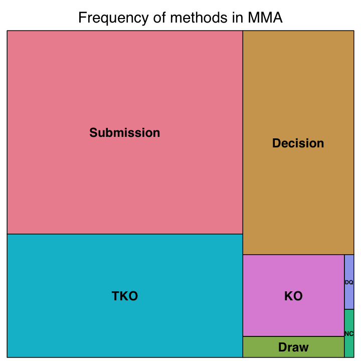
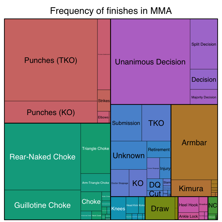
To visualize the frequency of methods and finishes, I will use treemaps generated using the treemap R package. A treemap visualizes the frequency of categories based on the area of a rectangle that they occupy (a category at 25% will occupy 25% of the total area). One nice feature about treemaps is that they can easily display hierarchical information. This won’t be useful for methods, but finishes can be grouped into subcategories to improve visualization.
library(treemap)

methods <- finish_types %>%
  select(Method = Method_cleanup, n) %>%
  count(Method, wt = n)

treemap(methods,
index = "Method",
vSize = "n",
title = "Frequency of methods in MMA",
fontsize.labels = 25, fontsize.title = 30)
finishes <- finish_types %>%
  select(Category = General_finish, Finish = Finish_cleanup, n) %>%
  count(Category, Finish, wt = n)

treemap(finishes,
index = c("Category", "Finish"),
vSize = "n",
title = "Frequency of finishes in MMA",
fontsize.labels = c(0, 25), fontsize.title = 30)
By visualizing finishes, we can see that the majority of finishes fall into a relatively small number of categories. The most common specific finishes were punches (a massive category that was split into TKO, KO and submission to provide some resolution), unanimous decision and three major submissions (Armbar, RNC and Guillotine). The most common classes of finishes were punches, followed by chokes and then decision. The fourth largest class was essentially miscellaneous finishes, a class that primarily pertains to fights where a specific finish was not recorded.
Now that we have cleaned up the results of our MMA matches, in my next post, I will discuss how we can clean up the data on individual fighters. This will help shed light on the demographics of MMA fighters, focusing on where MMA fighters live and the relative frequency of different weight classes.
Stay tuned, because in a couple weeks, I will revisit this finishes dataset. In this post, we grouped all wins into 50 well-defined categories. Individual fighters do not tend to use all types of finishes but tend to specialize in a subset of correlated finishes. Looking at the cooccurence of pairs of finishes, we can get a high level picture of the major MMA styles.