MMA styles II: ranking the top striking, submission and decision specialists
20 Dec 2016Ranking athletes is a common problem across all sports. In Mixed Martial Arts (MMA), one of the most popular ways of summarizing fighters is based on their primary method of winning. The major winning methods are: (1) KO/TKO: a fighter uses punches, kicks, etc. to either incapacitate the opponent (KO) or force a stoppage (TKO), (2) Submission: through chokes or joint locks a fighter forces his/her opponent to tap out, (3) Decision: the fight goes its full length and a panel of judges declare the winner.
The relative value of these three win methods is an important summary of a fighter’s style which is both reported by UFC’s pre-fight summary and is one of Sherdog’s main summaries of a fighter. Despite the importance of win method preference for summarizing fighters, it is difficult to rank fighters by their method preferences (the % of all wins by each method); using this metric, amateur fighters (with few wins to date) will often appear to be more specialized than experienced fighters. For example, a fighter who has won 3/3 times using strikes would appear to exclusively win by striking, while a fighter with 49/50 wins by striking would seem less specialized. Clearly, the latter fighter is probably a stronger striker because he/she has repeatedly demonstrated this preference, whereas there is more uncertainty about the former fighter.
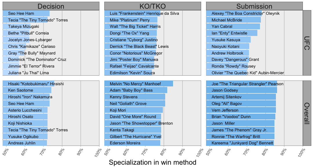
Here, I formalize this intuition by balancing fighter-specific results with patterns across fighters using a statistical approach based on empirical Bayesian analysis: a hierarchical Dirichlet-Multinomial model. Using this approach, I can fairly rank fighters accounting for their variable experience. Based on these experience-corrected rankings, Conor McGregor and Cris Cyborg are among the top 10 striking specialists in the UFC (K1 veteran Melvin Manhoef is top overall). Ronda Rousey and Dominick Cruz are top 10 in the UFC for winning by submission and decision, respectively.
Summarizing Raw Data
In a previous blog post, I presented a breakdown of >250,000 MMA fights in terms of methods (e.g., KO, TKO or submission) and finishes (e.g., armbar or punches). From this data, I summarized each fighter in terms of counts of each of the 3 methods of interest (KO/TKO, Submission and Decision).
library(mmadb)
suppressPackageStartupMessages(library(magrittr))

n_wins_threshold <- 4L # only look at fighters with >= 4 wins

fighter_win_methods <- mmadb::all_bouts %>%
  # look at wins
  dplyr::filter(Result == "win") %>%
  dplyr::group_by(Fighter_link) %>%
  # filter to fighters with more than n_wins_treshold wins
  dplyr::filter(n() >= n_wins_threshold) %>%
  # filter Methods that are not TKO, KO, Submission or Decision (e.g. NC or not reported: NA)
  dplyr::filter(Method_overwrite %in% c("TKO", "KO", "Submission", "Decision")) %>%
  # combine TKO and KO into KO/TKO
  dplyr::mutate(Method_overwrite = ifelse(Method_overwrite %in% c("TKO", "KO"), "KO/TKO", Method_overwrite)) %>%
  dplyr::select(Fighter_link, Method = Method_overwrite)

knitr::kable(fighter_win_methods %>%
  # count instances of each win method for each fighter
  dplyr::count(Fighter_link, Method) %>%
  tidyr::spread("Method", "n", fill = 0) %>%
  dplyr::ungroup() %>%
dplyr::sample_n(10))| Fighter_link | Decision | KO/TKO | Submission |
|---|---|---|---|
| /fighter/Jon-Hill-38397 | 0 | 10 | 2 |
| /fighter/Povilas-Markevicius-4340 | 1 | 0 | 4 |
| /fighter/Jarrett-Wainohu-62716 | 1 | 1 | 2 |
| /fighter/Niko-Lohmann-43694 | 0 | 1 | 5 |
| /fighter/Yuichiro-Yajima-12923 | 0 | 2 | 17 |
| /fighter/Glauber-Duncan-Santiago-174139 | 2 | 0 | 2 |
| /fighter/Josh-Tyler-73391 | 2 | 1 | 4 |
| /fighter/Petr-Vacek-85491 | 2 | 2 | 1 |
| /fighter/Mike-Marrello-17807 | 5 | 1 | 8 |
| /fighter/Alfred-Khashakyan-133919 | 0 | 8 | 0 |
To start thinking about how to analyze this data, it is useful to do some exploratory visualization. Because I am interested in each fighter’s relative investment in the three methods (KO/TKO, Submission, Decision), ternary diagrams are an attractive visualization approach. Ternary diagrams plot the relative value of three categories (e.g. \(x, y, z\)), constrained to sum to one (\(x + y + z = 1\)), within a triangle where proximity to each corner indicates the relative affinity for that category. I will use a ternary diagram to visualize each fighter’s counts of KO/TKO, submissions and decisions normalized to the sum of these three variables. I also stratify the partitions of fighters based upon experience (# of fights informing the estimate).
# visualize raw method counts

fighter_mle <- fighter_win_methods %>%
  # count instances of each win method for each fighter
  dplyr::count(Fighter_link, Method) %>%
  dplyr::group_by(Fighter_link) %>%
  dplyr::mutate(Pr_method = n/sum(n)) %>%
  dplyr::select(-n) %>%
  tidyr::spread("Method", "Pr_method", fill = 0)

# bin by n_wins_threshold
fighter_mle <- fighter_mle %>%
  dplyr::left_join(
    fighter_win_methods %>%
      dplyr::count(Fighter_link) %>%
      dplyr::mutate(bin = "# fights: <7",
                    bin = ifelse(n >= 7, "# fights: 7-12", bin),
                    bin = ifelse(n >= 13, "# fights: 13-20", bin),
                    bin = ifelse(n > 20, "# fights: >20", bin),
                    bin = ordered(bin, levels = c("# fights: <7", "# fights: 7-12", "# fights: 13-20", "# fights: >20"))) %>%
      dplyr::select(Fighter_link, bin),
    by = "Fighter_link")

suppressWarnings(suppressPackageStartupMessages(library(ggtern)))

# count unique occurences of decision, KO/TKO, submission for each bin (since these will not be unique in many cases)
dks_partition_counts <- fighter_mle %>%
  dplyr::ungroup() %>%
  dplyr::count(Decision, `KO/TKO`, Submission, bin)

dks_partition_counts <- dks_partition_counts %>%
  dplyr::rename(Dec = Decision,
                Sub = Submission)

ggtern(dks_partition_counts, aes(x = Dec, y = `KO/TKO`, z = Sub, color = n)) +
  geom_mask() +
  geom_point(size = 1.2) +
  facet_wrap(~ bin, ncol = 2) +
  scale_color_continuous("Number of fighters\nwith value", low = "royalblue1", high = "red", trans = "log10") +
  suppressWarnings(limit_tern(1.05, 1.05, 1.05)) +
  theme(text = element_text(size = 22))
There are only a small number of distinct combinations of methods that an inexperienced fighters could have won by (\(3^{n}\)). Accordingly, many fighters have either exclusively won by a single method or have won by only two of the three possible methods. Transitioning to more experienced fighters, most fighters have a method proportion that is not on the boundary of the ternary diagram. For these experienced fighters, observed method proportions should be a fairly accurate estimate of a fighter’s future win methods. That is, observed method proportions accurately estimate \(\Pr(\text{Method|Fighter})\). The method proportions of inexperienced fighters are more dubious predictors of this quantity because they overfit to observed win methods, thereby discounting that considerable uncertainty about these fighters exists.
To allow for fair estimation of fighters’ method preferences (\(\Pr(\text{Method|Fighter})\)) without regard to their level of experience, we can balance fighter-specific data with broader trends across fighters by estimating the distribution of methods (\(\Pr(\text{Method})\)) and utilizing this as a prior on the fighter-specific estimates. This prior will encompass both how common each method is and the extent to which fighters are method specialists (residing near the corners of the ternary diagram) or generalists (residing near the center of the ternary diagram).
Sharing information across fighters using a hierarchical model
Fighters’ win methods can be summarized by the \(I \times K\) matrix \(\mathbf{N}\) containing counts of each win method (\(k \in 1, 2, 3\)) by each fighter (\(i \in 1, 2, …, I\)). These counts can be thought of as drawn from fighter-specific Multinomial distributions parameterized by \(\theta_{i.}\). The Multinomial distribution is frequently used to represent data like dice rolls, but we generally don’t assume that each side is equally prevalent; instead, we are interested in estimating side probabilities. Due to the nature of this data, \(\theta\)s sum to 1 across the \(K = 3\) categories for each fighter \(i\), and \(\theta_{ik}\) equals the expected probability of the \(k\)th method for the \(i\)th fighter. In order to share information across fighters, we assume that these fighter-specific proportions are drawn from a single prior distribution. (This is why it’s called a hierarchical model.) A logical prior to place on the multinomially distributed fighter data is a Dirichlet distribution. Because the Dirichlet distribution is a conjugate prior to the Multinomial, the distributions can be cleanly combined to generate a closed form solution for the posterior (which will be the same distribution as the prior).
\[n_{i.} \sim \text{Multi}(\theta_{i.}, \sum{n_{i.}})\\ \theta_{i.} \sim \text{Dir}(\alpha_{1}, \alpha_{2}, \alpha_{3})\]This hierarchical Dirichlet-Multinomial relationship combines the Multinomial, which behaves like rolling a weighted \(K\) sided die, with the Dirichlet which adds $\alpha_{k}$ pseudocounts to each fighter’s record’s count of that method. Adding the \(\alpha\) pseudocounts to an inexperienced fighter will shrink their estimated \(\Pr(\text{Method|Fighter})\) towards the overall frequency of methods, while this addition will not greatly impact an experienced fighter with a large amount of data.
To further clarify how the Multinomial and Dirichlet will work together, we can consider that the Dirichlet-Multinomial distribution is a generalization of the Beta-Binomial from two categories (e.g. yes and no) to an arbitrary number of categories, \(K\). For a good resource on this distribution, Dave Robinson has nicely explained the importance of applying a Beta prior on Binomial baseball batting data (hits/total pitches) on his blog. As another example of Beta-Binomial, we can consider estimating a coin’s \(\Pr(\text{heads})\). If we flip a single coin 20 times and obtain 15 heads and 5 tails, the observed \(\Pr(\text{heads})\) is pretty far from the fair expectation (i.e. \(\Pr(\text{heads}) = 0.5\)). But, we should also assume that most coins are fair unless the data strongly overrules our assumption. Because of our strong prior assumptions regarding the behavior of coins, we should put a Beta prior on \(\Pr(\text{heads|flips})\) with fairly big parameters (lets say that its parameters \(\alpha\) and \(\beta\), which are equivalent to the \(\alpha\) parameters in the Dirichlet-Multinomial, are each 10). Because of the form of the Beta-Binomial, when we combine the prior and posterior, our posterior estimate of \(\Pr(\text{heads|flips})\) will have an expectation of \(\frac{H + \alpha}{H + \alpha + T + \beta} = \frac{15 + 10}{15 + 10 + 5 + 10} = 0.625\). Thus, we have shrunken our small amount of data on a single coin towards the behavior of coins overall.
One of the cool things about conjugate distributions like the Beta-Binomial and Dirichlet-Multinomial is that we can cleanly combine the prior and likelihood (of data, having assumed parameters), updating our prior belief based upon data. So, if we had some strong belief about the values of \(\alpha\), then we could update our estimate of \(\Pr(\text{Method|Fighter})\), encompassing this prior belief (the form of this update will be very similar to the coin example). Another cool property of the Dirichlet-Multinomial is that if we do not know the \(\alpha\) values and instead want to estimate these prior hyperparameters, we can integrate over fighter’s \(\theta\)s so that we can directly relate the support for our observed data (\(N\)) given the hyperparameters on our prior (\(\alpha\)s).
\[\Pr(\mathbf{N}|\mathbf{\alpha}) = \int_{\Theta}\Pr(\mathbf{N}|\Theta)Pr(\Theta|\mathbf{\alpha})d\Theta\\ \Pr(\mathbf{N}|\mathbf{\alpha}) = \prod_{i}\frac{\Gamma(A)}{\Gamma(N_{i} + A)}\prod_{k=1}^{K}\frac{\Gamma(n_{ik} + \alpha_{k})}{\Gamma(\alpha_{k})}\\ \log(\Pr(\mathbf{N}|\mathbf{\alpha})) = \sum_{i}\left[\log(\Gamma(A)) - \log(\Gamma(N_{i} + A)) + \sum_{k=1}^{K}\left[\log(\Gamma(n_{ik} + \alpha_{k})) - \log(\Gamma(\alpha_{k}))\right]\right]\\ \log(\Pr(\mathbf{N}|\mathbf{\alpha})) = I\left[\log(\Gamma(A)) -\sum_{k=1}^{K}\log(\Gamma(\alpha_{k}))\right] + \sum_{i}\left[- \log(\Gamma(N_{i} + A)) + \sum_{k=1}^{K}\log(\Gamma(n_{ik} + \alpha_{k}))\right]\]Here, \(A = \sum_{k}^{K}\alpha\) and \(N_{i} = \sum_{k}^{K}n_{ik}\). The second step is a known property of the Dirichlet-Multinomial. The third step log-transforms the marginal joint probability such that individual terms in the expression can be separately calculated without worrying about the product numerically rounding to zero. The fourth step refactors the summation so that it can be easily calculated during optimization. From this final expression, it is straightforward to determine the overall probability of our dataset for a given set of \(\alpha\) parameters. To instead determine optimal \(\alpha\) values given the dataset (the inverse problem), different sets of \(\alpha\) values can be proposed and evalutated using Markov Chain Monte Carlo (MCMC) in order to hone in on values of \(\alpha\) that best agree with our observed data.
Solving for prior parameters using MCMC
In order to find optimal values \(\alpha\), I used Metropolis-Hastings MCMC to identify a set of \(\alpha\) parameters sets that should (asymptotically) approximate the true distribution of \(\alpha\)s. At each step of the algorithm, I updated a single one of the \(\alpha\) values using a Gamma proposal distribution (leave the other \(\alpha\)s as is). The support for this proposal parameter set (\(\log(\Pr(\mathbf{N}|\mathbf{\alpha}^{\text{proposed}}))\)) was then compared to the current parameter set (\(\log(\Pr(\mathbf{N}|\mathbf{\alpha}^{\text{current}}))\)) and the proposal set replaced the current set if the proposed set was better supported. Otherwise, each parameter set (current and proposed) was accepted proportional to its probability.
fighter_total_counts <- fighter_win_methods %>%
  dplyr::count(Fighter_link) %>%
  dplyr::rename(fighter_n = n)

fighter_method_counts <- fighter_win_methods %>%
  dplyr::count(Fighter_link, Method) %>%
  dplyr::rename(method_n = n)

# Metropolis Hastings MCMC based estimation of alphas

multi_dirich_logLik <- function(fighter_total_counts, fighter_method_counts, alphas){
  count_w_prior <- fighter_method_counts %>%
    dplyr::left_join(alphas, by = "Method") %>%
    dplyr::mutate(n_plus_a = method_n + alpha)

  # only depend on alpha/A
  nrow(fighter_total_counts)*(lgamma(sum(alphas$alpha)) - sum(lgamma(alphas$alpha))) +
  # depends on N and A
  sum(-1*lgamma(fighter_total_counts$fighter_n + sum(alphas$alpha))) +
  # depends on method counts and a
  sum(lgamma(count_w_prior$n_plus_a))
}

gamma_shape <- 0.5
gamma_rate <- 0.5

# initialize
alphas_current <- tibble::data_frame(Method = unique(fighter_win_methods$Method)) %>%
  dplyr::mutate(alpha = rgamma(n = n(), shape = gamma_shape, rate = gamma_rate))
current_logLik <- multi_dirich_logLik(fighter_total_counts, fighter_method_counts, alphas_current)

n_steps <- 4000

logLik_track <- rep(NA, floor(n_steps/20))
alpha_track <- list()

for(i in 1:n_steps){
  for(j in 1:nrow(alphas_current)){
  # propose parameters
  alphas_proposed <- alphas_current
  alphas_proposed$alpha[j] <- rgamma(n = 1, shape = gamma_shape, rate = gamma_rate)

  # find logLikelihood of alphas | data
  proposed_logLik <- multi_dirich_logLik(fighter_total_counts, fighter_method_counts, alphas_proposed)

  if(runif(1, 0, 1) < exp(proposed_logLik - current_logLik)){
    alphas_current <- alphas_proposed
    current_logLik <- proposed_logLik
    }
  }
  logLik_track[i] <- current_logLik

  if(i %% 20 == 0){
    # record every 20th sample (we'll trash the early samples later as a burnin)
    logLik_track[i/20] <- current_logLik
    alpha_track[[i/20]] <- alphas_current %>%
      dplyr::mutate(sample = i/20)
    #print(paste(i, "steps done"))
  }
}

alpha_track <- alpha_track %>%
  dplyr::bind_rows()

# calculate the MAP estimate of alpha
alpha_posterior <- alpha_track %>%
  dplyr::left_join(tibble::data_frame(logLik = logLik_track) %>%
                     dplyr::mutate(sample = 1:n()),
                   by = "sample") %>%
  dplyr::group_by(Method) %>%
  dplyr::arrange(desc(logLik)) %>%
  dplyr::slice(1)

# compare alpha proportions to method proportions
method_breakdown <- alpha_posterior %>%
  dplyr::ungroup() %>%
  dplyr::mutate(alpha_frac = alpha/sum(alpha)) %>%
  dplyr::left_join(
    fighter_win_methods %>%
      dplyr::ungroup() %>%
      dplyr::count(Method) %>%
      dplyr::mutate(Method_fraction = n/sum(n)) %>%
      dplyr::select(-n),
    by = "Method")

knitr::kable(method_breakdown %>% dplyr::select(Method, `Method Proportion` = Method_fraction, alpha, `alpha Proportion` = alpha_frac) , digits = 3)| Method | Method Proportion | alpha | alpha Proportion |
|---|---|---|---|
| Decision | 0.234 | 1.273 | 0.261 |
| KO/TKO | 0.334 | 1.617 | 0.332 |
| Submission | 0.432 | 1.979 | 0.406 |
Using MCMC I generated a distribution of \(\mathbf{\alpha}\) parameter sets. From these samples, for the sake of convenience, I chose the MAP (the maximum posterior probability) estimate as a single consensus set of \(\alpha\) values. Inspecting the values of the MAP \(\alpha\)s, \(\alpha_{k}/\sum \alpha\) values are similar to \(\frac{\sum_{i}n_{ik}}{\sum_{ik}n_{ik}}\). This reveals that our prior has a similar shape to the popularity of individual methods, thereby adding weights of method to a fighter’s record based on the frequency of this method overall. The total magnitude of these \(\alpha\)s, 4.87, indicates how many total fights are effectively added to each fighter’s career.
Estimating \(\Pr(\text{Method|Fighter})\)
As was noted above for Beta-Binomial, the expected value of the posterior is the sum of the counts of an observation and the hyperparameter for this category (often called pseudocounts for this reason). The Dirichlet-Multinomial is no different. The posterior estimates for an individual fighter’s \(\Pr(\text{Method|Fighter})\) will be:
\[\mathbf{E}[\Pr(\text{Method}_{k}|\text{Fighter}_{i})] = \frac{n_{ik} + \alpha_{k}}{\sum_{ik'}n_{ik'} + \alpha_{k'}}\]These posterior probabilities can be used to identify which fighters are most specialized in each method.
# combine prior and likelihood to estimate each fighter's Pr(Method|Fighter)
fighter_Pr_method <- fighter_method_counts %>%
  tidyr::spread(Method, method_n, fill = 0) %>%
  tidyr::gather(Method, method_n, -Fighter_link) %>%
  # add the alpha prior weights to rows containing fighter-level counts for the corresponding method
  dplyr::left_join(alpha_posterior %>%
                     dplyr::select(Method, prior_counts = alpha),
                   by = "Method") %>%
  # sum counts of a method and prior counts to generate counts of the Dirichlet posterior
  dplyr::mutate(posterior_counts = method_n + prior_counts) %>%
  dplyr::group_by(Fighter_link) %>%
  dplyr::mutate(fighter_n = sum(method_n),
                Pr_method = round(posterior_counts/sum(posterior_counts), 3))

# add additional information about fighters: display name, and whether they have fought in UFC
top_fighter_stats <- fighter_Pr_method %>%
  dplyr::left_join(mmadb::fighter_vital_statistics, by = c("Fighter_link" = "Query")) %>%
  dplyr::select(Fighter_link, Display_name, Method, Pr_method, UFC)

# Find the fighter with the hightest Pr for each method overall and just for the UFC
top_fighter_stats <- top_fighter_stats %>%
    dplyr::mutate(UFC = "Overall") %>%
  dplyr::bind_rows(
    top_fighter_stats %>%
    dplyr::filter(UFC == "Current") %>%
    dplyr::mutate(UFC = "UFC")
  ) %>%
  # take the top 10 fighters in each method, in the UFC and overall
  dplyr::arrange(Method, UFC, desc(Pr_method)) %>%
  dplyr::group_by(Method, UFC) %>%
  dplyr::slice(1:10) %>%
  dplyr::mutate(rank = 1:n())

ranking_plot <- ggplot(data = top_fighter_stats %>%
         dplyr::ungroup() %>%
         dplyr::mutate(UFC = factor(UFC, levels = c("UFC", "Overall")))) +
  geom_bar(aes(x = rev(rank), y = Pr_method, fill = Pr_method), stat="identity") +
  geom_text(aes(x = rev(rank), label = Display_name), y = 0.51, hjust = 0, size = 5) +
  facet_grid(UFC ~ Method) +
  scale_y_continuous("Specialization in win method", labels = scales::percent, expand = c(0,0)) +
  scale_x_continuous(NULL, expand = c(0,0)) +
  scale_fill_gradientn(NULL, colors = c("slategray1", "skyblue2"), guide = "none") +
  coord_flip(ylim = c(0.48, 1)) +
  theme_minimal() +
  theme(panel.background = element_rect(color = "black", fill = "gray94"),
        strip.background = element_rect(fill = "gray70"),
        panel.grid.major = element_blank(),
        panel.grid.minor = element_blank(),
        panel.grid.major.x = element_line(size = 0.5, color = "gray70"),
        axis.ticks.x = element_line(size = 0.5, color = "gray70"),
        strip.text = element_text(size = 24),
        title = element_text(size = 24),
        axis.text.y = element_blank(),
        axis.text.x = element_text(size = 14, angle = 60, hjust = 1),
        panel.spacing = grid::unit(1.2, "lines"))

ranking_plot
Visualizing the prior on \(\Pr(\text{Method})\) and fighter-level estimates of \(\Pr(\text{Method|Fighter})\)
From the previous visualization of ternary diagrams, it was clear that inexperienced fighters were overfitted to their limited number of win methods. To see the effect of the above Bayesian analysis, I will again show the updated fighter method probabilities, laid upon the prior probability density. This prior can be thought of as representing the values that an individual fighter’s method probabilities can take (it is a distribution of distributions).
# summarize distribution of Pr(methods)
value_grid <- expand.grid(x = seq(0, 1, by = 0.01), y = seq(0, 1, by = 0.01)) %>%
  dplyr::mutate(z = 1 - x - y) %>%
  dplyr::filter(z >= 0)
colnames(value_grid) <- alpha_posterior$Method

value_grid$Pr_method <- apply(value_grid, 1, function(x){
  MCMCpack::ddirichlet(x, alpha = alpha_posterior$alpha)
})

method_breakdown_summary <- fighter_Pr_method %>%
  dplyr::select(Fighter_link, Method, Pr_method, fighter_n) %>%
  tidyr::spread(Method, Pr_method) %>%
  # bin by number of wins
  dplyr::mutate(bin = "# fights: <7",
                bin = ifelse(fighter_n >= 7, "# fights: 7-12", bin),
                bin = ifelse(fighter_n >= 13, "# fights: 13-20", bin),
                bin = ifelse(fighter_n > 20, "# fights: >20", bin),
                bin = ordered(bin, levels = c("# fights: <7", "# fights: 7-12", "# fights: 13-20", "# fights: >20"))) %>%
  dplyr::ungroup() %>%
  dplyr::count(bin, Decision, Submission, `KO/TKO`)

# cleanup methods for plotting
value_grid <- value_grid %>%
  dplyr::rename(Dec = Decision,
                Sub = Submission)

method_breakdown_summary <- method_breakdown_summary %>%
  dplyr::rename(Dec = Decision,
                Sub = Submission)

ggtern(value_grid, aes(x = Dec, y = `KO/TKO`, z = Sub)) +
  # background Pr distribution
  geom_point_swap(aes(fill = Pr_method)) +
  # Pr(method) for individual fighters
  geom_point(data = method_breakdown_summary, aes(color = n), size = 1) +
  scale_fill_gradientn("Pr(Method)", colors = c("gray90", "orange", "red")) +
  facet_wrap(~ bin, ncol = 2) +
  scale_color_continuous("Number of fighters\nwith value", low = "darkslategray1", high = "royalblue1", trans = "log10") +
  theme(text = element_text(size = 22))
In MMA, a large amount of data exists when pooling across fighters, but there is a more modest amount of fighter-specific data. By finding an empirical prior on method probabilities, fighters’ win methods were balanced with common trends across fighters. Inexperienced fighters are pulled towards a consensus of fighters, while experienced fighters are barely influenced by the prior. This will be an important element of future approaches, where instead of considering methods as a component of style, I will identify elements of style in a data-driven manner, capitalizing on common patterns in MMA finishes.
- Share this on →


