The not-so-small-world network of MMA fighters
17 May 2016There are over 140,000 amateur and professional mixed martial artists and the matchups between these fighters are far from random. It seems pretty obvious that Holly Holm’s next fight won’t be against Bigfoot Silva, but it is less clear how many reasonable matchups are out there for most fighters.
One way we can think about this question is that fighters will tend to compete against other fighters who are relatively similar to them. An amateur fighter may compete against fighters in his town and in neighboring towns. His opponents may do the same. While this fighter is unlikely to compete against fighters who live two towns over, he can still be said to be relatively closely connected to these fighters because they are only two jumps aways. At a broader scale, MMA fighters who are very different may be many jumps apart, seperated by large geographical barriers or other obstructions.
Looking at the matchups between pairs of fighters is the key to determining what drives these matchups overall. This analysis builds on past posts:
- Large-scale acquisition of fighter and fight data
- Quantitatively summarizing 240,000 MMA fights
- Summarizing the demographics of 140,000 MMA fighters
library(dplyr)

## Fighter-level data
fighters <- readRDS("~/Desktop/MMA/software/data/processed_fight_data/MMA_all_fighters.Rds")

kable(head(fighters %>% select(Display_name:Weight_class), 4), row.names = F)| Display_name | Record | Primary_affiliation | Gender | Nationality | Birthday | Height | Weight | Weight_class |
|---|---|---|---|---|---|---|---|---|
| Andrei “The Pit Bull” Arlovski | 25-11 (1 NC) | UFC (Current) | Male | Belarus | 1979-02-04 | 193.04 | 109.32 | Heavyweight |
| Ikuhisa “Minowaman” Minowa | 60-40-8 | PRIDE (Past) | Male | Japan | 1976-01-12 | 175.26 | 83.91 | Middleweight |
| Kazushi “The Gracie Hunter” Sakuraba | 26-17-1 (2 NC) | PRIDE (Past) | Male | Japan | 1969-07-14 | 182.88 | 75.75 | Welterweight |
| Ronda “Rowdy” Rousey | 15-1 | UFC (Current) | Female | United States | 1987-02-01 | 167.64 | 61.23 | Bantamweight |
## Fight-level data
bouts <- readRDS("~/Desktop/MMA/software/data/processed_fight_data/MMA_all_bouts.Rds")

# remove symmetrical pairs (i.e. only A-B, not A-B and B-A)
fighter_adjacency <- bouts %>%
  # count matchups between each fighter and all opponents
  count(Fighter_link, Opponent_link) %>%
  rowwise() %>%
  # by combining Fighter_link and Opponent_link and then sorting, A-B and B-A
  # will have the same Paired_link
  mutate(Paired_link = paste(sort(c(Fighter_link, Opponent_link)), collapse = "-")) %>%
  ungroup() %>%
  group_by(Paired_link) %>%
  # only take A-B or B-A, we only care about the link, not direction
  slice(1) %>% ungroup()

kable(head(fighter_adjacency, 4), row.names = F)| Fighter_link | Opponent_link | n | Paired_link |
|---|---|---|---|
| /fighter/1651-1651-40638 | /fighter/Akito-Oguchi-36825 | 1 | /fighter/1651-1651-40638-/fighter/Akito-Oguchi-36825 |
| /fighter/1651-1651-40638 | /fighter/Takuya-Takahashi-81447 | 1 | /fighter/1651-1651-40638-/fighter/Takuya-Takahashi-81447 |
| /fighter/2Face-2Face-67592 | /fighter/Tobizaru-Tobizaru-67593 | 1 | /fighter/2Face-2Face-67592-/fighter/Tobizaru-Tobizaru-67593 |
| /fighter/634-634-129431 | /fighter/Nobuyuki-Tanioka-128927 | 1 | /fighter/634-634-129431-/fighter/Nobuyuki-Tanioka-128927 |
Summary of MMA fight network
Matchups between fighters are reminiscent of six degrees of seperation, an idea that most people can be connected by six or less steps: a friend of a friend of … of a friend. The suprisingly close proximity of seemingly random pairs of individuals is a common feature of social networks. This property is even more pronounced for the facebook network; where random users are seperated by an average of 3.5 friends.
We can look at the connectivity of MMA matchups in a similar way to see how many steps are between the average pair of fighters. To address this question, we can consider bouts as undirected edges that connect fighters and the whole set of fighters and bouts as an undirected network. Using igraph we can easily calculate the number of jumps between every pair of fighters in this network.
library(igraph)

# turn the links between pairs of fighters into undirected edges
vital_graph <- graph_from_data_frame(fighter_adjacency, directed = F, vertices = fighters)

# delete small disconnected groups
graph_clusters <- clusters(vital_graph)
disconnected_fighters <- graph_clusters$membership[graph_clusters$membership %in% c(1:graph_clusters$no)[graph_clusters$csize < 100]]
vital_graph <- delete_vertices(vital_graph, which(V(vital_graph)$name %in% names(disconnected_fighters)))

# structural properties

network_mean_distance = mean_distance(vital_graph)
network_diameter = diameter(vital_graph)
In comparison with most social networks, fighters are only loosely connected. The average number of bouts seperating fighters is 8.4 and the longest distance between any two fighters is 38.
To see why there are such large distances between fighters, we can project demographic factors (fighters’ locations, genders, weight classes …) onto the matchup network.
Major factors affecting matchups
Thus far, we have considered the network of fighters (connected by bouts) which is defined solely by its connectivity. In order to visualize this network, we need to create a physical parallel between the network’s connectivity and the positions of fighters in physical space (i.e. each fighter has some [x,y] coordinates). While many approaches exist to produce such network layouts, the main goal of these approaches is to make it so that fighters who are closely connected in network space become closely connected in cartesian space. For this analysis, I will use the DRL force-directed layout algorithm, which is included in igraph. DRL works well on large datasets; it can generate a layout for this 150k node, 250k edge network in a couple of minutes.
Based on the network layout, we can expect that fighters who are closer together generally fight similar opponents. With this layout in hand, we can seperately project fighters’ weights, locale and gender onto the network to see how these factors affect matchups.
library(ggraph)

# layout fighters using the DRL layout (good for large graphs)
set.seed(1234)
vital_graph_xy <- layout_with_drl(vital_graph)
vital_graph_xy <- as.data.frame(vital_graph_xy)
colnames(vital_graph_xy) <- c("x", "y")

# generate a ggraph object with node coordinates (for ggplot2-based plotting)
gg_vital_graph <- createLayout(vital_graph, layout = "manual", node.positions = vital_graph_xy)

# theme for network plots
graph_theme <- theme_minimal() + theme(axis.text = element_blank(), panel.grid = element_blank(), axis.title = element_blank(), legend.key.size = unit(0.5, "inches"), legend.text = element_text(size = 12), legend.title = element_text(size = 15), plot.background = element_rect(fill = "white", color = "white"), text = element_text(color = "black"), strip.background = element_rect(color = "gray50"), plot.title = element_text(size = 20))ggraph(data = gg_vital_graph) +
geom_node_point(aes(color = Nation_region), size = 1, alpha = 0.5) +
graph_theme + guides(colour = guide_legend(override.aes = list(size = 8, alpha = 1))) +
scale_color_manual("Region", limits = region_colors$Nation_region,
values = region_colors$Region_color) +
ggtitle("Fighters colored by geographical region (based on nationality)")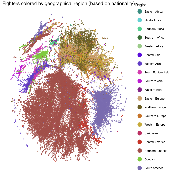
ggraph(data = gg_vital_graph) +
  geom_node_point(aes(color = Weight_class), size = 1, alpha = 0.5) +
  graph_theme +
  scale_colour_gradientn("Weight Class", colours = rainbow(7),
                         breaks = 1:length(levels(fighters$Weight_class)),
                         labels = levels(fighters$Weight_class)) +
  ggtitle("Fighters colored by weight class")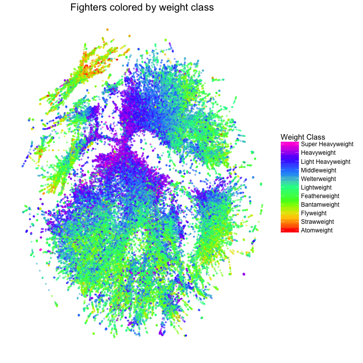
ggraph(data = gg_vital_graph) +
  geom_node_point(aes(color = Gender), size = 1, alpha = 0.5) +
  graph_theme + guides(colour = guide_legend(override.aes = list(size = 8, alpha = 1))) +
  scale_color_brewer("Gender", palette = "Set1") +
  ggtitle("Fighters colored by gender (based on first name)")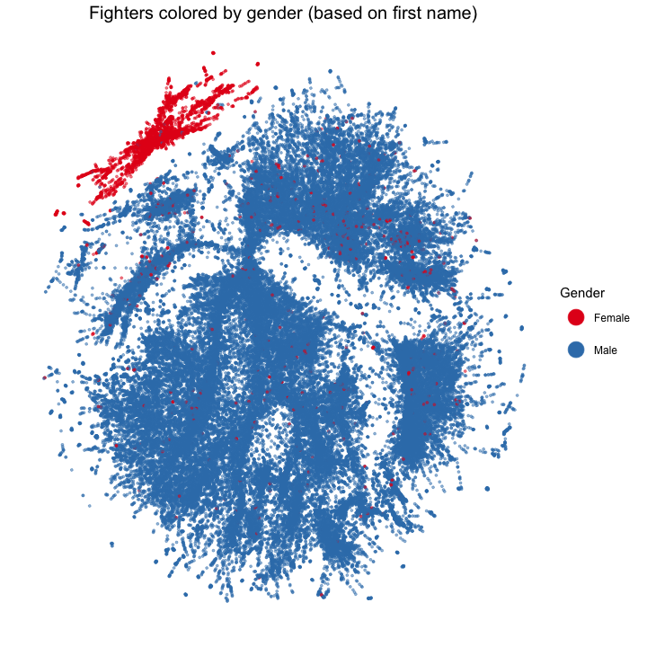
Having looked at weight class, locale and gender, we can see that each attribute partially explains this network’s diffuse structure.
The regions where fighters come from structure the global fighter network into geographical blocks. Central American fighters are sandwiched between North American fighters and south american fighters. European fighters form a coherent group, although there is some finer structure, with regions of the graph that primarily contain Northern or Eastern European fighters. Asian countries form the other major cluster which also include Oceania: primarily Australia and New Zealand.
Weight class polarizes each region with one side primarily lighter weight classes and the other side largely heavier weight classes. Interestingly, the heaviest weight classes converge at the intersection of the major geographical categories, suggesting that heavy European, Asian and American fighters are more likely to compete than lighter fighters. This is likely because there are many more light fighters than heavy fighters so heavy fighters have an easier time making it onto the international scene.
Gender is another factor that majorly structures the fighter network. A note on this plot: because fighter genders were inferred by virtue of first names (and connectivity), the isolated pockets of red fighters in the blue network and blue in the red are likely just mislabelled. Male and female fighters form seperated subnetworks due to the almost total absence of cross-gender competition (interestingly, these graphs are connected).
With these three factors, we can explain the major trends in the network layout; however, this summary doesn’t give us a full idea of the distances seperating fighters.
Understanding the distances between fighters
From the plots of geography, weight classes and gender, it seems that fighters are resolved into fairly tight groups by virtue of these three factors. While the diameter of this network (8.4) is large for a social network, it still seems small relative to the strong factors that structure fighters. To understand how two random fighters can be linked with only ~8 jumps, we need to consider how large differences in demographics are efficiently bridged by the network.
A likely way that such long distance jumps can be accomplished is through the top athletes of the sport. Top fighters have had many opponents, likely changed weight classes across their career and may have fought against athletes from other continents. Two methods of visualizing these top athletes should illustrate how these fighters can operate as hubs to facilitate long distance jumps.
Coloring top fighters within the original network
top_fighers <- fighters %>% filter(UFC != "None" | Bellator != "None" | WSF != "None" | PRIDE != "None")

# highlight UFC, WSF and Bellator fighters
gg_vital_graph$top <- ifelse(V(vital_graph)$name %in% top_fighers$Query, T, F)

ggraph(data = gg_vital_graph) +
  geom_node_point(aes(alpha = top, colour = top), size = 1) +
  graph_theme +
  scale_colour_manual("Tier", limits = c(T,F), values = c("RED", "BLACK"), labels = c("Top", "Rest")) +
  scale_alpha_manual("Tier", limits = c(T,F), values = c( 0.5, 0.02), labels = c("Top", "Rest")) +
  guides(colour = guide_legend(override.aes = list(alpha=1, size = 8))) +
  ggtitle("Highlighting ~2,000 UFC, WSF, PRIDE and Bellator fighters")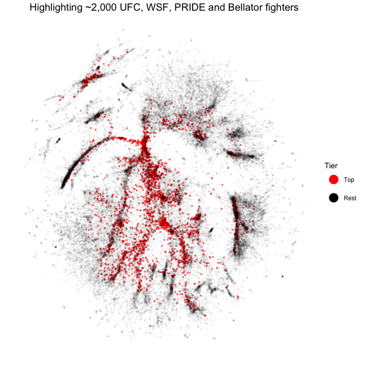
Coloring top fighters within their own network
top_vital_graph <- delete_vertices(vital_graph, which(!(V(vital_graph)$name %in% top_fighers$Query)))

top_vital_graph_xy <- layout_with_drl(top_vital_graph)
top_vital_graph_xy <- as.data.frame(top_vital_graph_xy)
colnames(top_vital_graph_xy) <- c("x", "y")

top_gg_vital_graph <- createLayout(top_vital_graph, layout = "manual", node.positions = top_vital_graph_xy)

ggraph(data = top_gg_vital_graph) +
  geom_node_point(aes(color = Weight_class,
                      Name = Display_name,
                      Nationality = Nationality,
                      WC = Weight_class), size = 1, alpha = 0.5) +
  graph_theme +
  scale_colour_gradientn("Weight Class", colours = rainbow(7),
                         breaks = 1:length(levels(fighters$Weight_class)),
                         labels = levels(fighters$Weight_class)) +
  ggtitle("Just looking at ~2,000 top fighters")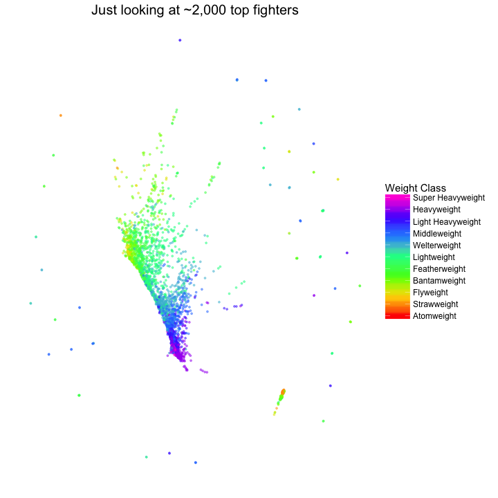
Looking at top fighters within our original layout, we see that their location is influenced by the same types of factors as all other MMA fighters: they form groups that are clustered according to weight class, locale and gender.
This structure is markedly different if we only look at a network composed of these top fighters. When only looking at top fighters, the primary factors that influence who-fights-who are weight class and gender. Note that this graph is more disconnected then when looking at all fighters: there is a subgraph for the major male fighters, the major female fighters, as well as many small groups of fighters who are not connected to the larger groups.
The difference between these two plots owes to the different phases of a top-tier MMA fighter’s career. All fighters have to start somewhere, so they will likely have multiple matches against fighters from their homeland. As they progress to higher-level competition, they will compete against more diverse opponents.
This suggests a model that could connect a random pair of fighter (F1 and F2): short range jumps connect F1 to an international fighter, jumps among international fighters traverse differences in weight class and locale, and another set of short range jumps ultimately reach F2. We can test this by visualizing the shortest paths connecting a set of random fighters
Visualizing the paths between fighters
# Choose npaths random pairs of vertices
npaths <- 5
set.seed(123)
fighter_pairs <- sapply(1:npaths, function(x){sample(V(vital_graph)$name, 2)})

# find the shortest path between each pair
random_pairs <- lapply(1:npaths, function(x){
  get.shortest.paths(vital_graph, fighter_pairs[1,x], fighter_pairs[2,x], mode = "all", output = "both")
})

# find the coordinates of fighters in the sequence
track_nodes <- lapply(1:npaths, function(x){data.frame(set = x, fighter_seq = as_ids(random_pairs[[x]]$vpath[[1]]))}) %>%
  bind_rows %>%
  group_by(set) %>%
  mutate(step_num = 1:n())

track_nodes_ids <- data.frame(fighter_seq = V(vital_graph)$name[V(vital_graph)$name %in% track_nodes$fighter_seq],
vital_graph_xy[V(vital_graph)$name %in% track_nodes$fighter_seq,])

track_nodes <- track_nodes %>% left_join(track_nodes_ids, by = "fighter_seq")

# find the coordinates of the edges
track_edges <- lapply(1:npaths, function(x){data.frame(set = x, get.edges(vital_graph, random_pairs[[x]]$epath[[1]]))}) %>% bind_rows

track_edges_coords <- data.frame(set = factor(track_edges$set),
           x = vital_graph_xy$x[track_edges$X1],
           xend = vital_graph_xy$x[track_edges$X2],
           y = vital_graph_xy$y[track_edges$X1],
           yend = vital_graph_xy$y[track_edges$X2])

# for repelling text
library(ggrepel)

ggraph(data = gg_vital_graph) +
  geom_node_point(aes(alpha = top, colour = top), size = 1) +
  geom_edge_link(data = track_edges_coords, aes(x = x, xend = xend, y = y, yend = yend, colour = set, group = set), edge_width = 2) +
  geom_label_repel(data = track_nodes, aes(x = x, y = y, label = step_num, fill = factor(set)), color = "black", size = 5) +
  graph_theme +
  scale_colour_manual("Tier", limits = c(T,F), values = c("RED", "BLACK"), labels = c("Top", "Rest")) +
  scale_alpha_manual("Tier", limits = c(T,F), values = c( 0.5, 0.02), labels = c("Top", "Rest")) +
  guides(colour = guide_legend(override.aes = list(alpha=1, size = 8))) +
  scale_edge_colour_brewer("Random fighter pairs", palette = "Set2") +
  scale_fill_brewer("Random fighter pairs", palette = "Set2") +
  ggtitle("Paths between random pairs of fighters")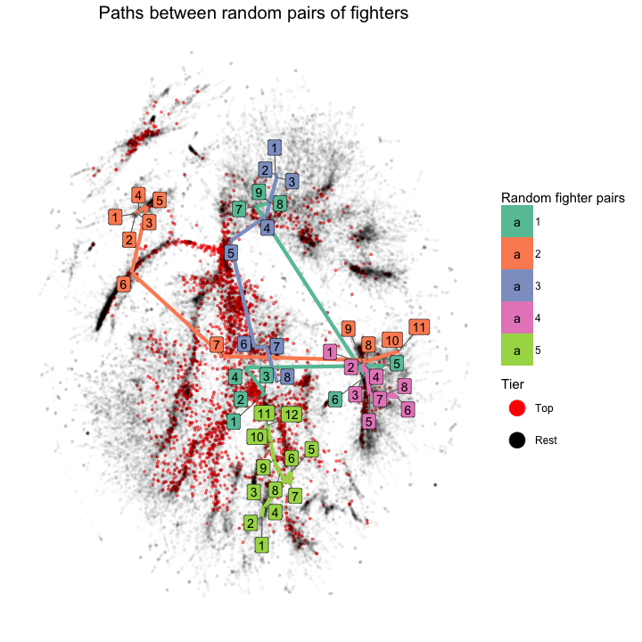
Looking at a set of representative paths between random fighters, we see the pattern that I suggested above emerge: fighters usually require multiple jumps to reach well-connected fighters; these well-connected fighters make distant jumps across weight classes and regions; finally, the destination fighter also likely requires several local jumps.
Two factors contribute to the not-so-small-world network of MMA fighers: the relatively low number of connections of most fighters (leading to short local jumps to reach hubs), and broad demographic differences among fighters (requiring long distance jumps across demographics). The great distances between fighters are primarily due to low connectivity; all social networks contain barriers, and the MMA network is an extreme but likely not unprecedented example. Nevertheless, these barriers clearly impose a strong structure on the MMA fighting community where competitions are greatly structured based on geography, weight, gender and experience.